Home    Site Map    Path Curves (1)    Path Curves (2)    Path curves(3)
See, also, the downloadable Word documents,
 (1) Practical Path Curve Calculations by N.C. Thomas
 (2) Practical Bud Observation              by G. Calderwood       (Web version here)
 (3) Practical Bud Measurement     also by G. Calderwood       (Web version here)
(3) describes manual, rather than computer-assisted, methods, so should be of use to those without a PC!
Fitting a Path Curve:  the Math of the Method

tetrahedron_view

The General Approach

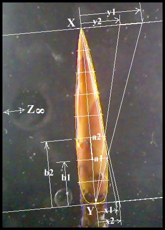
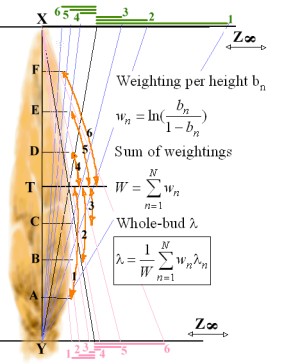
The bud is fitted into an invariant triangle, XYZ, then measured at N heights, 7 in this case, as depicted on the left, on a Beech bud.

Vertex X is called the Top Pole, and vertex Y is called the Bottom Pole.

 Then, to find λ, ( t is the stepping parameter)—

  • take the IPD (inter-pole distance) as 1.0
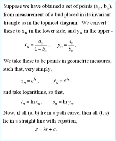
  • find x and y from a and b by simple proportion
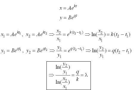
  • take points x and points y as points in geometric progressions with multipliers k and q respectively
Then use—

Thus, λ is just the ratio of the characteristic multipliers, q and k, of the two geometric progressions.

We obtain a list of λ s for the number of levels at which we have chosen to measure the bud, and take their mean value to be the value of λ for the whole bud.  If the bud were a perfect path curve, and if we were able to measure the bud with perfect precision, all the values in the list would be the same.  In practice, there is variation, and we can use various statistical methods to cope with it.

We may of course choose to let variable a represent the measurements of radii, left or right, or of diameters. (The terms arise from the approximately-circular, horizontal cross-section of a bud.)

There are several specific methods* of analysis.  Two are
available in the Bud Workshop program
[* needs references]

(a) The Projective Method


This method was devised by Lawrence Edwards.  The bud's IPD is evenly divided at an odd number of "fractional" heights (usually seven), so that a height (labelled T on the diagram on the left) is always available exactly half way between the poles. All estimates of λ are referred to this central height.  Thus, as shown left, λ-estimate number 1 would pertain to the portion of the profile of the bud lying between level A and T (here indicated by the arrowed orange arc, marked, '1'), λ-estimate number 2 to the profile between B and T, (here marked, '2'), and so on, giving for the total number N of  λ-estimates one fewer than the total number of heights.

Now, the λ-estimates for portions of the profile near to the central height are obviously extremely susceptible to measurement-error. Edwards used the rather ingenious weighting scheme shown on the diagram to mitigate this vulnerability, together with the corresponding whole-bud λ formula, also shown. 

(b) The Regression Method


This method
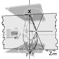
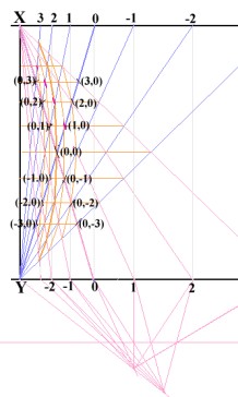
was devised by Graham Calderwood.  It regards the measures in the invariant triangle as co-ordinates, equivalent to so-called "ordinary", Cartesian co-ordinates. Indeed, it is easily shown that Cartesian co-ordinates are a special, very restricted case of these co-ordinates, so they are in fact extra-ordinary!.  The "layout" of the co-ordinate grid, or graticule,  is as shown on the left.

The equation of a path curve reckoned with respect to these co-ordinates is identical to that of a straight line reckoned with respect to ordinary, Cartesian co-ordinates, namely -

                    s = λt + c

Where t is the independent variable (the stepping parameter, as above), and  c and λ are constants.

In other words, a path curve is a straight line in its own frame of reference - which is, for buds and eggs, the semi-imaginary invariant tetrahedron.  (The invariant triangle in which we set the real bud is an "axial section" through this tetrahedron.)

  • The slope of this line is our 'shape factor', λ.
  • The intercept, c, is an indication of the "disposition" of the bud in its own space, and a measure of its size in "ordinary" space.
The elliptical, orange path curves shown above have a slope (that is, λ) of +1.0. The bold curve passes through the origin.  The straight, horizontal, orange lines are path curves with a slope, or λ , of -1.0.  In their own "bud space", these sets of path curves lie at right angles to each other.

So the business of finding the path curve best matching a real bud reduces to finding a straight line of  best fit, and the well-known, well-worn, statistical technique called linear regression is ideally suited to the task.  Hence the name given to the method.
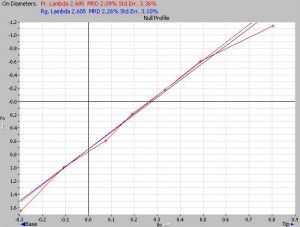
null_graph

On the left is the graph in "bud space", on seven diameters, for the beech bud shown above. The red line is the straight-line fit by the projective method. The blue line is the fit by the regression method. The bud shows a reasonable fit over its profile, except at the topmost and bottommost heights. Such mismatches often indicate that

  • The poles are poorly placed, or
  • The bud is perhaps opening, or
  • There are too few measurements.
Signage
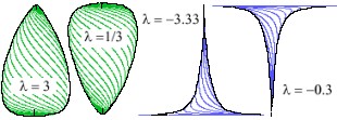
It will be noticed that the numbers are flagged (signed) oppositely on the two horizontal limbs or sides of the triangle (those connecting to the Z vertex at infinity).  Negatives are on the right on the top limb, and on the left on the bottom limb.  This is done simply for convenience, to ensure that the λ of an egg-shaped profile comes out positive. If such a λ is fractional (0.0 <= λ < 1.0), the egg/bud is "sharp end down".  If λ is exactly unity (1.0), the form is equally rounded at both ends - it is an ellipse or a circle. Otherwise, it is "sharp end up".
Correspondingly, by this convention, a vortex-profile has a negative λ , and if in this case |λ| is a fraction, the "throat" of the vortex lies in the bottom pole. If |λ| is unity, it lies in neither pole (the path curve profile is a horizontal, straight line terminating somewhere on the XY axis). Otherwise, it lies in the top pole.

If we regard the throat of a vortex as the "sharp" end of it (it surely looks sharp!), then we may say that the sharp ends of egg and vortex with the same |λ| share one pole, and the "blunt" ends share the other.  Notice, also, that the curves pass between just two of the vertices of the triangle, and avoid the third.  Finally, notice that forms that are identical, but inverted with respect to each other, have λs that are reciprocals of each other - so to invert the λ is to invert the form, and vice versa.
Home    Site Map    Path Curves (1)    Path Curves (2)    Path Curves(3)